SocialGraphs
Draft of Social Graphs report.
Содержание
Social Random Graphs Models
Introduction
Recently there has been much interest in studying large-scale real-world networks and attempting to model their properties using random graphs. Although the study of real-world networks as graphs goes back some time, recent activity perhaps started with the paper of Watts and Strogatz [WattsStrogatz1998] about the ‘small-world phenomenon’.
Since then the main focus of attention has shifted to the ‘scale-free’ nature of the networks concerned, evidenced by, for example, power-law degree distributions.
It was quickly observed that the classical models of random graphs introduced by Erdős and Rényi [ErdosRenyi1959] and Gilbert [Gilbert1956] are not appropriate for studying these networks, so many new models have been introduced.
One of the most rapidly growing types of networks are social networks.
Social networks are defined as a set of actors or network members whom are tied by one or more type of relations.
The actors are most commonly persons or organizations however they could be any entities such as web pages, countries, proteins, documents, etc. and sometimes under a more general name, information networks.
There could also be many different types of relationships, to name a few, collaborations, friendships, web links, citations, information flow, etc.
These relations represented by the edges in the network connecting the actors and may have direction (shows the flow from one actor to the other) and strength (shows how much, how often, how important).
Recently, following an interest in studying social networks structure among mathematicians and physicists, researchers investigated statistical properties of networks and methods for modeling networks either analytically or numerically.
It was observed that in many networks the distribution of nodes degrees is highly skewed with a small number of nodes having an unusually large degrees.
Moreover they observed that degree sequences of such networks satisfyied so-called 'power-low'.
This means that the probability of a node to have degree k is equal to , where parameter characterises concrete type of networks.
The work in studying such networks falls very roughly into the following categories.
- Direct studies of the real-world networks themselves, measuring various properties such as degree-distribution, diameter, clustering, etc.
- Introdusing new random graph models motivated by this study.
- Computer simulations of the new models, measuring their properties.
- Heuristic analysis of the new models to predict their properties.
- Rigorous mathematical study of the new models in order to prove theorems about their properties.
Although many interesting papers have been written in this area (see, for example, the survey [AlbertBarabasi2002]), so far almost all of this work comes under 1-4. To date there has been little rigorous mathematical work in the field.
In the rest of this chapter we briefly mention the classical models of random graphs and state some results about these models chosen for comparison with recent results about the new models. Then we consider the scale-free models and note that they fall into two types.
The first takes a power-law degree distribution as given, and then generates a graph with this distribution. The second type arises from attempts to explain the power law starting from basic assumptions about the growth of the graph. We will consider models of second type preferably.
We describe
- the Barabási-Albert (BA) model,
- the LCD model, a generalization due to Buckley and Osthus [BuckleyOsthus2001],
- the copying models of Kumar, Raghavan, Rajagopalan, Sivakumar, Tomkins and Upfal [KumarRaghavan2000],
- the very general models defined by Cooper and Frieze [CooperFrieze2003].
Concerning mathematical results we concentrate on the degree distribution, presenting results showing that the models are indeed scale-free and briefly discuss results about properties other than degree sequence: the clustering coefficient, the diameter, and ‘robustness’.
Classical models of random graphs
The theory of random graphs was founded by Erdős and Rényi in a series of papers published in the late 1950s and early 1960s.
Erdős and Rényi set out to investigate what a ‘typical’ graph with n labelled vertices and M edges looks like.
They were not the first to study statistical properties of graphs; what set their work apart was the probabilistic point of view: they considered a probability space of graphs and viewed graph invariants as random variables.
In this setting powerful tools of probability theory could be applied to what had previously been viewed as enumeration questions.
The model of random graphs introduced by Gilbert [Gilbert1956] (precisely at the time that Erdős and Rényi started their investigations) is, perhaps, even more convenient to use.
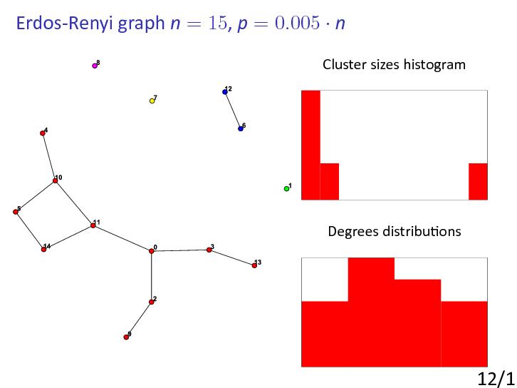
Let Gn,p be the random graph on n nodes in which two nodes i and j are adjacent (connected by an edge) with probability p (independently of all other edges).
So, to construct a random , put in edges with probability p' independently of each other.
It is important that p is often a function of n, though the case p constant, 0 < p < 1, makes perfect sense.
The important study is so-called 'evolution' of random graphs Gn,p that is the study for what functions some parameters or properties of random graphs appear ([ErdosRenyi1960]).
We are interested in what happens as n goes to infinity and we say that Gn,p has a certain property P with high probability (whp) if the probability that Gn,p has this property tends to 1.
For example, it was shown that if then component structure depends on the value of c.
If c < 1 then whp every component of Gn,p has order .
If c > 1 then whp Gn,p has a component with nodes, where a(c) > 0 and all other components have nodes.
Another observation was made for the degree sequence ditribution.
If with c>0 constant the probability of node to have degree k is asyptotically equal to as n goes to infinity (so-called Poisson distribution).
It was proved that in wide range of the diameter of is asymptotic to
For many other important properties (connectivity, perfect matchings, hamiltonicity, etc) similar results was proved as well.
Many other interesting results in classical probabilistic models of random graphs can be found in [JansonLuczakRucinski2000].
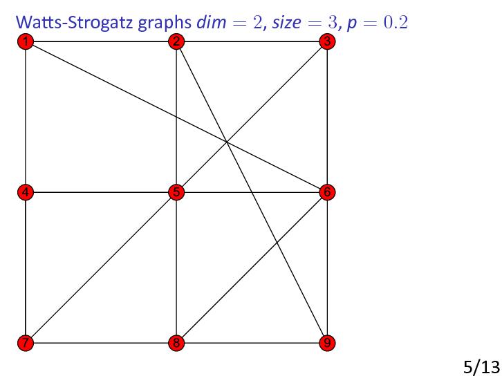
Watts-Strogatz model
In 1998, Watts and Strogatz [WattsStrogatz1998] raised the possibility of constructing random graphs that have some of the important properties of real-world networks.
The real-world networks they considered included
- neural networks,
- the power grid of the western United States
- the collaboration graph of film actors.
Watts and Strogatz noticed that these networks were ‘small-world’ networks: their diameters were considerably smaller than those of regularly constructed graphs (such as lattices, or grid graphs) with the same number of vertices and edges.
More precisely, Watts and Strogatz found that real-world networks tend to be highly clustered, like lattices, but have small diameters, like random graphs.
That large social networks have rather small diameters had been noticed considerably earlier, in the 1960s, by Milgram [Milgram1967] and others, and was greatly popularized by Guare’s popular play ‘six degrees of separation’ in 1990.
The importance of the Watts and Strogatz paper is due to the fact that it started the active and important field of modelling large-scale networks by random graphs defined by simple rules.
As it happens, from a mathematical point of view, the experimental results in [WattsStrogatz1998] were far from surprising. Instead of the usual diameter diam(G) of a graph G, Watts and Strogatz considered the average distance.
As pointed out by Watts and Strogatz, many real-world networks tend to have a largish clustering coefficient and small diameter. To construct graphs with these properties, Watts and Strogatz suggested starting with a fixed graph with large clustering coefficient and ‘rewiring’ some of the edges. It was shown that introduction of a little randomness makes the diameter small.
Scale-free models
In 1999, Faloutsos, Faloutsos and Faloutsos [Faloutsos1999] suggested certain ‘scale-free’ power laws for the graph of the Internet, and showed that these power laws fit the real data very well.
In particular, they suggested that the degree distribution follows a power law, in contrast to the Poisson distribution for classical random graphs Gn,p.
This was soon followed by work on rather vaguely described random graph models aiming to explain these power laws, and others seen in features of many real-world networks.
In fact, power-law distributions had been observed considerably earlier; in particular, in 1926 Lotka claimed that citations in academic literature follow a power law, and in 1997 Gilbert suggested a probabilistic model supporting Lotka's law.
The degree distribution of the graph of telephone calls seems to follow a power law as well; motivated by this, Aiello, Chung and Lu [AielloChungLu2001] proposed a model for massive graphs.
This model ensures that the degree distribution follows a power law by fixing a degree sequence in advance to fit the required power law, and then taking the space of random graphs with this degree sequence.
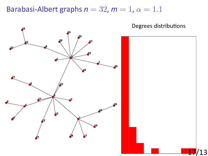
The Barabási-Albert model
Perhaps the most basic and important of the scale-free random graph models, i.e., models producing power-law or scale-free behaviour from simple rules, is the BA model.
This was introduced by Barabási and Albert in [AlbertBarabasi1999]:
- ... starting with a small number m0 of vertices,
- at every step we add a new vertex with m edges that link the new vertex to m different vertices
already present in the system assume that the probability P that a new vertex will be connected to a vertex i depends on the connectivity ki of that vertex, so that .
- After t steps the model leads to a random network with t + m0 vertices and mt edges.
The basic motivation is to provide a highly simplified model of the growth of, for example, the world-wide web.
New sites (or pages) are added one at a time, and link to earlier sites chosen with probabilities depending on their current popularity — this is the principle that «popularity is attractive».
Barabási and Albert themselves, and many other people, gave experimental and heuristic results about the BA model.
The Buckley-Osthus model
Two groups,
- Dorogovtsev, Mendes and Samukhin [DorogovtsevMendesSamukhin2000]
- Drinea, Enachescu and Mitzenmacher [DrineaEnachescuMitzenmacher2001],
introduced a variation on the BA model in which vertices have an initial attractiveness: the probability that an old vertex is chosen to be a neighbour of the new vertex is proportional to its in-degree plus a constant initial attractiveness, which we shall write as .
The case is just the BA model, since there total degree is used, and each out-degree is m.
The LCD model
The LCD (linearized chord diagram) proposed in [BollobasRiordan2000] has a simple static description and very useful for obtaining mathematical results for scale-free graphs.
In [BollobasRiordan2001] it was proved that random graphs generated according the LCD model are indeed scale-free graphs.
In fact in [BollobasRiordan2004] it was proved that the diameter of scale-free graphs in this model is asymptotically in contrast to known conjecrute (based on experiments) that the diameter is for some constant c.
The copying model
Around the same time as the BA model, Kumar, Raghavan, Rajagopalan, Sivakumar, Tomkins and Upfal [KumarRaghavan2000] gave rather different models to explain the observed power laws in the web graph. The basic idea is that a new web page is often made by copying an old one, and then changing some of the links.
The linear growth copying model is parametrized by a copy factor and a constant out-degree d > 1.
- At each time step, one vertex u is added, and u is then given d out-links for some constant d.
- To generate the out-links, we begin by choosing a prototype vertex p uniformly at random from Vt (the old vertices).
The i-th out-link of u is then chosen as follows.
- With probability α, the destination is chosen uniformly at random from Vt, and with the remaining probability the out-link is taken to be the i th out-link of p.
- Thus, the prototype is chosen once in advance.
The d out-links are chosen by -biased independent coin flips, either randomly from Vt, or by copying the corresponding out-link of the prototype.
The intuition behind this model is the following.
When an author decides to create a new web page, the author is likely to have some topic in mind. The choice of prototype represents the choice of topic—larger topics are more likely to be chosen. The Bernoulli copying events reflect the following intuition: a new viewpoint about the topic will probably link to many pages «within» the topic (i.e., pages already linked to by existing resource lists about the topic), but will also probably introduce a new spin on the topic, linking to some new pages whose connection to the topic was previously unrecognized.
As for the BA model, it was proved that the degree distribution does follow a power law and the probability of node to have degree k is asymptotically
.
The Cooper-Frieze model
Recently, Cooper and Frieze [CooperFrieze2003] introduced a model with many parameters which includes the last three models as special cases, and proved a very general result about the power-law distribution of degrees. In the undirected case, the model describes a (multi-)graph process G(t), starting from G(0) a single vertex with no edges. Their attachment rule is a mixture of preferential (by degree) and uniform (uniformly at random, or ‘u.a.r’).
Initially, at step t = 0, there is a single vertex . At any step t = 1, 2, ..., T, ... there is a birth process in which either new vertices or new edges are added.
Specifically, either a procedure NEW is followed with probability , or a procedure OLD is followed with probability .
In procedure NEW, a new vertex v is added to G(t − 1) with one or more edges added between v and G(t − 1).
In procedure OLD, an existing vertex v is selected and extra edges are added at v.
The recipe for adding edges typically permits the choice of initial vertex v (in the case of old) and the terminal vertices (in both cases) to be made either u.a.r or according to vertex degree, or a mixture of these two based on further sampling. The number of edges added to vertex v at step t by the procedures (NEW, OLD) is given by distributions specific to the procedure.
The details of these choices are to complicated to be presented here and depend on a lot of parameters.
The results say that the ‘expected degree sequence’ converges in a strong sense to the solution of a certain recurrence relation, and that under rather weak conditions, this solution follows a power law with an explicitly determined exponent and a bound on the error term. Cooper and Frieze also prove a simple concentration result, which we will not state, showing the number of vertices of a certain degree is close to its expectation.
One of the basic properties of the scale-free random graphs considered in many papers is the clustering coefficient C. This coefficient describes ‘what proportion of the acquaintances of a vertex know each other’.
Formally, given a simple graph G (without loops and multiple edges), and a vertex v (with at least two neighbours, say), the local clustering coefficient at v is the number of edges between neighbours of v divided by the number of all possible edges between neighbours of v. The clustering coefficient for the whole graph is the average of local clustering coefficients over all verticies of a graph.
Robustness and vulnerability
Another property of scale-free graphs and the real-world networks inspiring them which has received much attention is their robustness.
Suppose we delete vertices independently at random from G, each with probability q.
- What is the structure of the remaining graph?
- Is it connected?
- Does it have a giant component?
A precise form of the question is: fix 0 < q < 1.
Suppose vertices of G are deleted independently at random with probability q = 1 − p.
Let the graph resulting be denoted Gp.
For which p is there a constant c = c(p) > 0 independent of n such that with high probability Gp has a component with at least cn vertices?
The answer to this natural question was obtained in [BollobasRiordan2003]: with high probability the largest component of Gp has order c(p)n for some constant c(p) > 0.
However, it turns out that this giant component becomes very small as p approaches zero and has order
Conclusions
There is a great need for models of real-life networks that incorporate many of the important features of these systems, but can still be analyzed rigorously. The models defined above are too simple for many applications, but there is also a danger in constructing models which take into account too many features of the real-life networks. Beyond a certain point, a complicated model hardly does more than describe the particular network that inspired it. In fact some balance between simplicity of model and correspondence to real-life social networks is needed.
If the right balance can be achieved, well constructed models and their careful analysis should give a sound understanding of growing networks that can be used to answer practical questions about their current state, and, moreover, to predict their future development.
References
- [AielloChungLu2001] W. Aiello, F. Chung and L. Lu, A random graph model for power law graphs, Experiment. Math. 10 (2001), 53-66.
- [AlbertBarabasi2002] R. Albert and A.-L. Barabási, Statistical mechanics of complex networks, Rev. Mod. Phys. 74 (2002), 47-97.
- [AlbertBarabasi1999] A.-L. Barabási and R. Albert, Emergence of scaling in random networks, Science 286 (1999), 509—512.
- [BollobasRiordan2000] B. Bollobas and O.M. Riordan, Linearized chord diagrams and an upper bound for Vassiliev invariants, J. Knot Theory Ramifications 9 (2000), 847-853.
- [BollobasRiordan2003] Bollobas B., Riordan O.M., Robustness and vulnerability of a scale-free random graph, Internet Mathematics, 2003, v. 1, N 1, p. 1-35.
- [BollobasRiordan2004] Bollobas B., Riordan O.M., The diameter of a scale-free random graph, Combinatorica, 2004, v. 24, N 1, p. 5-34.
- [BollobasRiordan2001] B. Bollobas, O. Riordan, J. Spencer and G. Tusn´ady, The degree sequence of a scale-free random graph process, Random Structures and Algorithms 18 (2001), 279—290.
- [BuckleyOsthus2001] Buckley, P.G. and Osthus, D., Popularity based random graph models leading to a scale-free degree sequence, Discrete Mathematics, 2001, volume 282, 53-68
- [CooperFrieze2003] C. Cooper and A. Frieze, A general model of web graphs, Journal Random Structures & Algorithms, Volume 22 Issue 3, May 2003
- [DrineaEnachescuMitzenmacher2001] E. Drinea, M. Enachescu and M. Mitzenmacher, Variations on random graph models for the web, technical report, Harvard University, Department of Computer Science, 2001.
- [DorogovtsevMendesSamukhin2000] S.N. Dorogovtsev, J.F.F. Mendes, A.N. Samukhin, Structure of growing networks with preferential linking Phys. Rev. Lett. 85 (2000), 4633.
- [ErdosRenyi1959] Erdős, P., and Rényi, A., On random graphs I., Publicationes Mathematicae Debrecen 5 (1959), 290—297.
- [ErdosRenyi1960] Erdős, P., and Rényi, A., On the evolution of random graphs, Magyar Tud. Akad. Mat. Kutat´o Int. K¨ozl. 5 (1960), 17-61.
- [Faloutsos1999] M. Faloutsos, P. Faloutsos and C. Faloutsos, On power-law relationships of the internet topology, SIGCOMM 1999, Comput. Commun. Rev. 29 (1999), 251.
- [Gilbert1956] Gilbert, E.N., Enumeration of labelled graphs, Canad. J. Math. 8 (1956), 405—411.
- [JansonLuczakRucinski2000] Janson, S., Luczak, T., and Rucinski, A. (2000). Random Graphs. John Wiley and Sons, New York, xi+ 333pp.
- [KumarRaghavan2000] R. Kumar, P. Raghavan, S. Rajagopalan, D. Sivakumar, A. Tomkins and E. Upfal, Stochastic models for the web graph, FOCS 2000.
- [Milgram1967] Milgram, S., The small world phenomenon, Psychol. Today 2 (1967), 60-67.
- [NewmanStrogatzWatts2001] M.E.J. Newman, S.H. Strogatz and D.J. Watts, Random graphs with arbitrary degree distribution and their applications, Physical Review E 64 (2001), 026118.
- [WattsStrogatz1998] D. J. Watts and S. H. Strogatz, Collective dynamics of small-world networks, Nature 393 (1998), 440—442.
- [NewmanPark2003] M. Newman, J. Park, Why social networks are different from other types of networks, Phys. Rev. E, 2003, v. 68, P036122.
- [LibenNovak2005] D. Liben-Nowell, J. Novak, R. Kumar, P. Raghavan, A. Tomkins, Geographic routing in social networks, Proc. of the National Academy of Sciences, 2005, v. 102(33), p. 11623-11628.
Community detection and clusterization
Social network analysis examines the structure and composition of ties in the network to answer different questions like:
- Who are the central actors in the network?
- Who has
- the most outgoing connections?
- the most incoming connections?
- the least connections?
- How many actors are involved in passing information through the network?
- Which actors are communicating more often with each others?
The question we are focused here is how one can find communities in a given social network?
First we will list the important terms in a social network analysis and then we will summarize the work related to a community detection in social networks.
- Neighborhood
- of a node consists of its adjacent nodes i.e. the nodes directly connected to it by an edge.
- Clique
- is a subgraph of a network where all the actors are connected to each other.
- Density
- is a measure for how connected the actors are in a network i.e. the proportion of ties in the network divided by the total number of possible ties.
The important question we will address in the rest of this section is how difficult to find communities in a graphs? In fact, the answer depends on formal definition of a community. Today there has not been any consensus on the exact definition of community. Informally speaking the community is a densely connected subset of nodes that is only sparsely linked to the remaining network, a subgraph which is more tightly connected than average. There are different ways to formalize this notion.
The following target function is often used to measure quality of resulting partition of the graph into communities and defines so-called modularity Q of the partition which evaluates the density of links inside communities as compared to links between communities:
where
- Aij represents the weight of the edge between vertexes i and j,
- , is the community to which vertex i is assigned,
- is 1 if u=v and 0 otherwise,
- .
There are other definitions of modularity and quality of community partitions.
Finding a partition of the graph with maximum modularity is NP-hard problem [BrandesDellig2006]. An interesting open problem in this area is to study how good modularity can be efficiently approximated. It is important to stress that similar problems in graph theory (finding maximum clique or chromatic number in a graph) are difficult to approximate [Hastad97], [Hastad1997]. Moreover, such problems may be hard even in random graphs (see, [JuelsPeinado1998], [AlonKrivelevichSudakov1998].
Similar to the notion of community is the notion of a dense subgraph.
Given an undirected graph G = (V, E), the density of a subgraph on vertex set S is defined aswhere E(S) is the set of edges in the subgraph induced by S.
The problem of finding the densest subgraph of a given graph G can be solved optimally in polynomial time (using flow technique), despite the fact that there are exponentially many subgraphs to consider [Gpldberg1984]. In addition, Charikar [Charikar2000] showed that we can find a 2-approximation to the densest subgraph problem in linear time using a very simple greedy algorithm. This result is interesting because in many applications of analyzing social networks, web graphs etc., the size of an graph involved could be very large and so having a fast algorithm for finding an approximately dense subgraph is extremely useful.
However when there is a size constraint specified — namely find a densest subgraph of exactly k vertices, the densest k subgraph problem becomes NP-hard [FeigeKortsarzPeleg1997], [AsahiroHassinIwama2002].
Graph Partitioning Approaches
At first glance community detection seems close to graph partitioning problems in machine learning. Unfortunately one may not apply available methods for partititioning to the problem of community mining because of the assumptions on availability of predefined partition size, which is not a valid assumption for real social networks.
The objective of graph partitioning algorithms is to divide the vertices of the graph into k groups of predefined size, while minimizing the number of edges lying between these groups, called cut size [Fortunato2010]. Finding the exact solution in graph partitioning is known to be NP-complete.
However there are several fast but sub-optimal heuristics. The most well-known Kernighan-Lin algorithm [KernighanLin1970].
The Kernighan-Lin algorithm optimizes a benefit function Q, which represents the difference between the number of edges inside the groups and the number of edges running between them. It start by partitioning the graph into two groups of equal size and then swaps subset of vertices between these groups to maximize Q. After a series of swaps, it chooses the group with largest Q for partitioning in the next iteration.
This algorithm has time complexity where n is the number of vertices [Fortunato2010].
Another important family of graph partitioning algorithms is the spectral clustering methods [NgJordanWeiss2001]. They divide the network into groups using the eigenvectors of matrices, mostly the Laplacian matrix.
The major incompatibility of these methods is that community structure detection assumes that the networks divided naturally into some partitions and there is no reason that these partitions should be of the same size. In minimum cut methods, often it is necessary to specify both the number and the size of the groups.
If one tries to minimize the cut size without fixing the number of groups, the solution would be grouping all the vertices in one group.
Several alternatives measures have been proposed for the cut size, such as
- Conductance Cut
- Cut size divided by minimum of sum of degrees of vertices in C and outside C
- Ratio Cut
- Cut size divided by minimum of number of vertices in the subgraphs [ChanSchlagZien1993]
- Normalized Cut
- Cut size divided by sum of degrees of vertices in C [ShiMalik2000].
Hierarchical Clustering Approaches
Hierarchical clustering approaches define a similarity measure between vertices and group similar vertices together to discover the natural divisions in a given network.
Hierarchical clustering approaches classify into two major categories:
- agglomerative algorithms
- iteratively merge groups with high similarity
- divisive algorithms
- iteratively remove edges connecting vertices with low similarity.
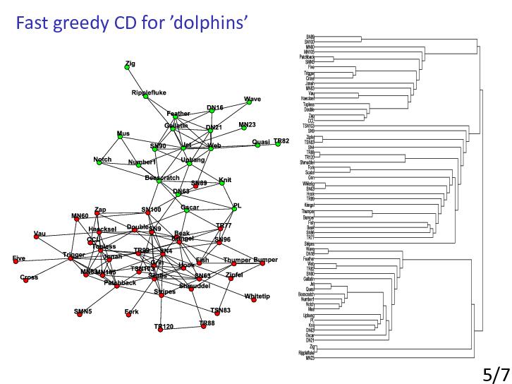
Well-known algorithm that uses hierarchical clustering was proposed by Girvan and Newman [GirvanNewman2002]. Their method is a divisive hierarchical clustering algorithm which iteratively removes the edge with highest betweenness to obtain community structure of the network.
The betweenness of an edge could be computed as the number of shortest paths running through that edge.
High betweenness is a sign for bridges in the network, which are edges connecting different communities.

Their approach obtains a good result in real world data sets, however, it is computationally expensive and unscalable for large networks as it needs running time of O(m2 n) in general and O(n3) in sparse networks, where m is the number of edges [GirvanNewman2002].
Modularity Based Approaches
The modularity Q as defined above is a measure for assessing communities which shows the quality of that particular partitioning of the network.
There are variety of approximate optimization algorithms for searching the space of possible partitionings of a network in order to detect the partitioning with the highest modularity.
Newman uses a greedy optimization in [NewmanGirvan2004]. He employs an agglomerative clustering method, starting with each vertex as a cluster, in each step it merges the clusters that most increase the modularity.
Later Clauset [ClausetNewman2004] presented a very fast version of the algorithm which has become very popular ever since.
A modification of the CNM algorithm [ClausetNewman2004] that treats newly combined communities as a single node after each iteration is able to identify community structure on a network containing 1 billion edges in a matter of hours.
Local algorithms
The more recent directions in community mining includes the investigation of local algorithms for very large networks, the detection of overlapping communities, and the examination of community dynamics.
The idea of LPA (label propagation) algorithm is to assign first each node in a network a unique label (that is all nodes are in different communities). Every iteration, each node is updated in a greedy manner by choosing the label which most of its neighbors have. If there are more than one maximum labels one of such labels is picked randomly. Clear advantage of label propagation is the fact that it can be parallelized easily.
A new fast algorithm is proposed in [BlondelGuillaume2008]. The algorithm is divided in two phases that are repeated iteratively. Assume that we start with a weighted network of N nodes.
- First, we assign a different community to each node of the network.
So, in this initial partition there are as many communities as there are nodes.
- Then, for each node i we consider the neighbors j of i and we evaluate the gain of modularity that would take place by removing i from its community and by placing it in the community of j.
- The node i is then placed in the community for which
this gain is maximum (in case of a tie use a breaking rule), but only if this gain is positive.
- If no positive gain is possible, i stays in its original community.
This process is applied repeatedly and sequentially for all nodes until no further improvement can be achieved and the first phase is then complete.
This first phase stops when a local maxima of the modularity is attained, i.e., when no individual move can improve the modularity.
The first part of the algorithm efficiency results from the fact that the gain in modularity ΔQ obtained by moving an isolated node i into a community C can easily be computed.
The second phase of the algorithm consists in building a new network whose nodes are now the communities found during the first phase.
To do so, the weights of the links between the new nodes are given by the sum of the weight of the links between nodes in the corresponding two communities.
Links between nodes of the same community lead to self-loops for this community in the new network.
Once this second phase is completed, it is then possible to reapply the first phase of the algorithm to the resulting weighted network and to iterate.
Let us denote by «pass» a combination of these two phases. The passes are iterated until there are no more changes and a maximum of modularity is attained.
This simple algorithm has several advantages. First, its steps are easy to implement, and the outcome is unsupervised. Moreover, the algorithm is extremely fast, i.e., computer simulations on large ad-hoc modular networks suggest that its complexity is linear on typical and sparse data.
It was reported that this algorithm has identified communities in a 118 million nodes network in 152 minutes [Fortunato2010].
Clustering
In some way community detection problem in real social networks is related to clustering problem which can be formulated as follows.
Given the set of n points in Rd and an integer k. The goal is to choose k centers from these n points so that to minimize the sum of the squared distances between each point and its closest center.
Social network can be considered as multidimensional space (if each node has a lot of parameters as in Facebook), thus clustering approach may be suitable.
Clustering problem is NP-hard even for k=2 [DrineasFrieze2004].
Very simple local search algorithm was proposed by Lloyd in 1982 [LLoyd1982].
This algorithm is also referred as k-means.
It is good algorithm in terms of speed, but it does not have any proven estimates for its solutions accuracy.
In 2007 [ArthurVassilvitskii2007] enhanced version of Lloyd's algorithm was proposed called k-means++.
It have been proven to be -competitive. Moreover, the algorithm is much faster than k-means and provides better clusterization in practice.
Like k-means this algorithm is fast and can be easily parallelized.
Overlapping communities
Algorithms, described above, produce non-overlapping partitions/communities, and this may be OK in homogeneous social networks, there all connections are professional contacts.
For example, there are good non-overlapping partition of local LinkedIn cluster («professional contacts» of one co-author of the report, forming a «bridge» between several professional communities):

But it is important to note that communities in common social networks (such as Facebook) are often overlapping but all algorithms described above finds only non-overlapping partition of vertices.
For example, none of several «out of box» community detection algorithms (GirvanNewman, Newman-Moore, Louvain, Wakita-Tsurumi) provide reasonable community detection in local Facebook cluster («friends» of one co-author of the report):

The reason of overlapping is based on obvious fact that in social networks all participants share several roles.
So it is desirable, that community detection of social graphs (such as Facebook) will use algorithms for overlapping communities.
Clique percolation
The clique percolation method ([PallaDerenyiFarkas2005]) builds up the communities from k-cliques. Two k-cliques are considered adjacent if they share k-1 nodes.
A community is defined as the maximal union of k-cliques that can be reached from each other through a series of adjacent k-cliques.
This definition allows overlaps between the communities in a natural way, see picture below.

Since even small networks can contain a vast number of k-cliques, the implementation of this approach is based on locating the maximal cliques rather than the individual k-cliques.
Thus, the complexity of this approach in practice is equivalent to that of the NP-complete maximal clique finding, (in spite that finding k-cliques is polynomial).
This means that although networks with few million nodes have already been analyzed successfully with this approach [PallaBarabasiVicsek2007] no prior estimate can be given for the runtime of the algorithm based simply on the system size.
Line graphs
Another new and prominent approach of overlapping community detection is edge partioning (so-called «line graphs») [EvansLambiotte2010].
The algorithm consists of three steps:
- Convert original graph to line graph (see picture), where
- each edge became a vertex in a line graph
- each vertice became a set of edges in a clique.

- Run some classical vertices-partitioning algorithm (may be parallel) on a (weighted) line graph to receive edge separation for original graph.
Conclusions
1. There are different definitions of communities.
It is important to stress that communities in social networks are often overlapping but this fact did not reflected in current definitions of modularity.
This is obvious fact, that in social networks all participants share several roles. So it is desirable, that community detection of social graphs (such as Facebook) use algorithms for non-overlapping communities (clique percolation, partitioning of edge graphs).
2. All community detection algorithms are heuristics.
It is important to have a measure how good approximation the algorithms can provide.
3. In view of very high size of social graphs (expected number of users in Facebook is about billion with average number of connections is 120 [FacebookDataminingSurvey2009]) only very fast heuristics can be considered as candidates mainly using local algorithms.
It seems interesting to apply ideas of good initial choice of k-centers in k-means++ to new fast local algorithms finding communities.
References — community and clustering
- [AlonKrivelevichSudakov1998] N. Alon, M. Krivelevich, B. Sudakov, Finding a large hidden clique in a random graph, Random Structures and Algorithms, 1998, v. 13, pp. 457--466.
- [AsahiroHassinIwama2002] Y. Asahiro, R. Hassin, and K Iwama. Complexity of finding dense subgraphs. Discrete Appl. Math., 121(1-3):15-26, 2002.
- [ArthurVassilvitskii2007] D. Arthur, S. Vassilvitskii. k-means++: the advantages of careful seeding. Proceedings of the eighteenth annual ACM-SIAM symposium on Discrete algorithms, P. 1027-1035, 2007.
- [BackstromHuttenlocher2006] Lars Backstrom, Dan Huttenlocher, Jon Kleinberg, and Xiangyang Lan. Group formation in large social networks: membership, growth, and evolution. In ACM SIGKDD, pages 44-54, 2006.
- [BlondelGuillaume2008] Vincent D. Blondel, Jean-Loup Guillaume, Renaud Lambiotte, Etienne Lefebvre. Journal of Statistical Mechanics: Theory and Experiment, V. 2008(10), 2008.
- [BrandesDellig2006] Brandes U, Delling D, Gaertler M, Goerke R, Hoefer M, Nikoloski Z and Wagner D, On Finding Graph Clusterings with Maximum Modularity, 2006.* [Charikar2000] M. Charikar. Greedy approximation algorithms for finding dense components in a graph. In APPROX, pages 84-95, 2000.
- [ChenZaianeGoebel2009] J. Chen, O. R. Zaiane, and R. Goebel. Local community identification in social networks. In Proceedings of the International Conference on Advances in Social Network Analysis and Mining(ASONAM), pages 237—242, 2009. http://webdocs.cs.ualberta.ca/~zaiane/postscript/SNAkdd10.pdf
- [Clauset2005] A. Clauset. Finding local community structure in networks. Physical Review E, 72:026132, 2005.
- [ClausetNewman2004] A. Clauset, M. E. J. Newman, and C. Moore. Finding community structure in very large networks. Phys. Rev. E, 70:066111, 2004.
- [DrineasFrieze2004] P. Drineas, A. Frieze, R. Kannan, S. Vempala, V. Vinay. Clustering large graphs via the singular value decomposition. Machine Learning, V. 56(1-3), P. 9-33, 2004.
- [EvansLambiotte2010] Evans, TS, Lambiotte R, Line Graphs of Weighted Networks for Overlapping Communities, European Physical Journal B
- [FeigeKortsarzPeleg1997] U. Feige, G. Kortsarz, and D. Peleg. The dense k-subgraph problem. Algorithmica, 29:410-421, 1997.
- [FlakeLawrenceGiles2000] G.W. Flake, S. Lawrence, and C. L. Giles. Efficient identification of web communities. In KDD, pages 150—160, 2000.
- [Fortunato2010] Santo Fortunato. Community detection in graphs. Physics Reports, 486(3-5):75 — 174, 2010.
- [FacebookDataminingSurvey2009] Maintained Relationships on Facebook, Report 2009, http://www.facebook.com/note.php?note_id=55257228858&ref=mf
- [Goldberg1984] A. V. Goldberg. Finding a maximum density subgraph. Technical report, 1984.
- [Hastad97] J. Hastad, Some optimal inapproximability results, STOC’97, Proc. of the 29th Annu. ACM Symposium on Theory of Computing.
- [Hastad1997] J. Hastad, Clique is hard to approximate within $n^{1-\varepsilon}$, Proceedings of the 37th Annual IEEE Symposium on Foundations of Computing, 1997, pp. 627-636.
- [JuelsPeinado1998] A. Juels, M. Peinado, Hiding Cliques for Cryptographic Security, Proceedings of the 9th Annual ACM-SIAM Symposium on Discrete Algorithms, 1998, pp. 678-684.
- [GirvanNewman2002] Michelle Girvan and M. E. J. Newman. Community structure in social and biological networks. In Proceedings of the National Academy of Science USA, 99:8271-8276, 2002.
- [Gregory2007] S. Gregory. An algorithm to find overlapping community structure in networks. In PKDD, pages 91-102, 2007.
- [KernighanLin1970] B. W. Kernighan and S. Lin. An efficient heuristic procedure for partitioning graphs. Bell System Technical Journal, 9:291-307, 1970.
- [LuoWangPromislow2006] F. Luo, J. Z. Wang, and E. Promislow. Exploring local community structures in large networks. In WI ’06: Proceedings of the 2006 IEEE/WIC/ACM International Conference on Web Intelligence, pages 233—239, 2006.
- [LLoyd1982] Stuart P. Lloyd. Least squares quantization in PCM. IEEE Transactions on Information Theory, V 28(2), P. 129-136, 1982.
- [NepuszPetrocziNegyessy2008] T. Nepusz, A. Petroczi, L. Negyessy, and F. Bazso. Fuzzy communities and the concept of bridgeness in complex networks. Physical Review E, 77, 2008.
- [Newman2004] M. E. J. Newman. Detecting community structure in networks. Eur. Phys. J.B, 38:321-330, 2004.
- [Newman2006] M. E. J. Newman. Modularity and community structure in networks. PROC.NATL.ACAD.SCI.USA, 103, 2006.
- [NewmanGirvan2004] M. E. J. Newman and M. Girvan. Finding and evaluating community structure in networks. Physical Review E, 69, 2004.
- [NgJordanWeiss2001] A. Ng, M. Jordan, and Y. Weiss. On spectral clustering: Analysis and an algorithm. In NIPS, pages 849—856, 2001.
- [PallaDerenyiFarkas2005] G. Palla, I. Derenyi, I. Farkas, and T. Vicsek. Uncovering the overlapping community structure of complex networks in nature and society. Nature, 435:814-818, 2005.
- [PallaBarabasiVicsek2007] G. Palla, A.-L. Barabási and T. Vicsek, Quantifying social group evolution, Nature, 446, 664–667(2007).
[ Хронологический вид ]Комментарии
Войдите, чтобы комментировать.